Since submitting my master’s thesis back in 2021, I wanted to do a quick postmortem on it in this blog - here goes, three years later.
After dabbling in GPGPU for a while, and already having touched on pointcloud CSG (or Booleans - terms vary), my master’s thesis tackled a significantly less attractive challenge this field poses: Performing CSG on triangle meshes, entirely on GPU.
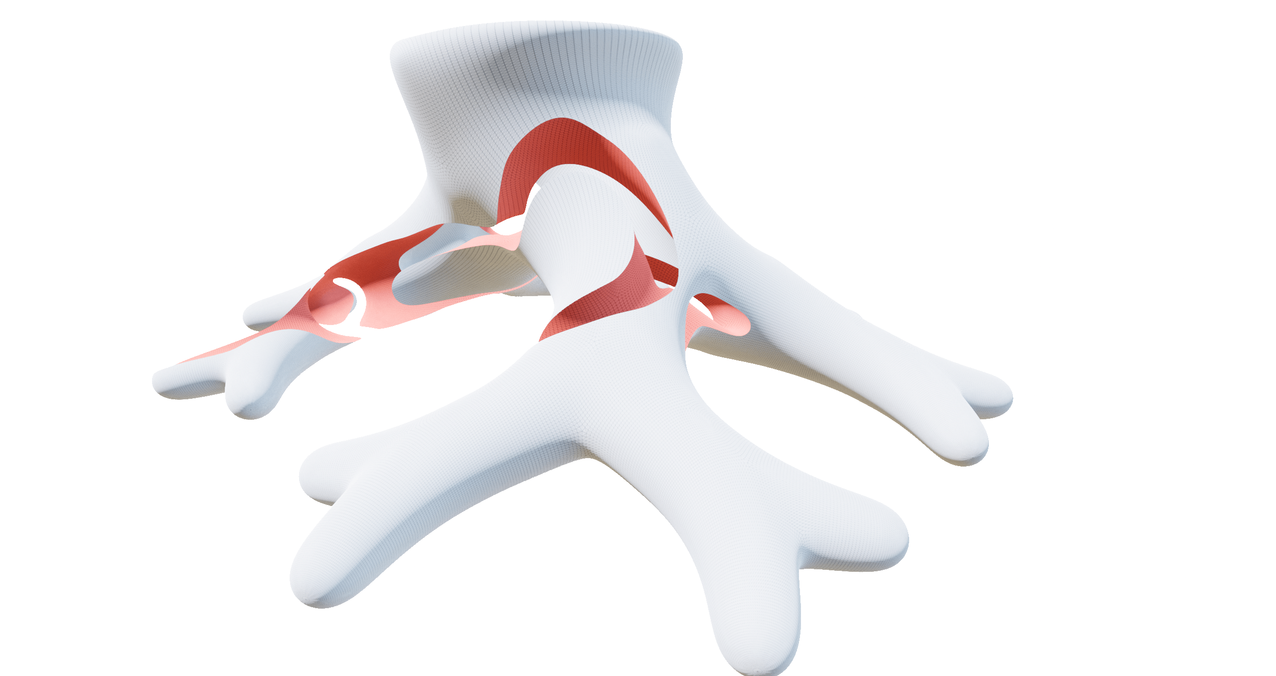
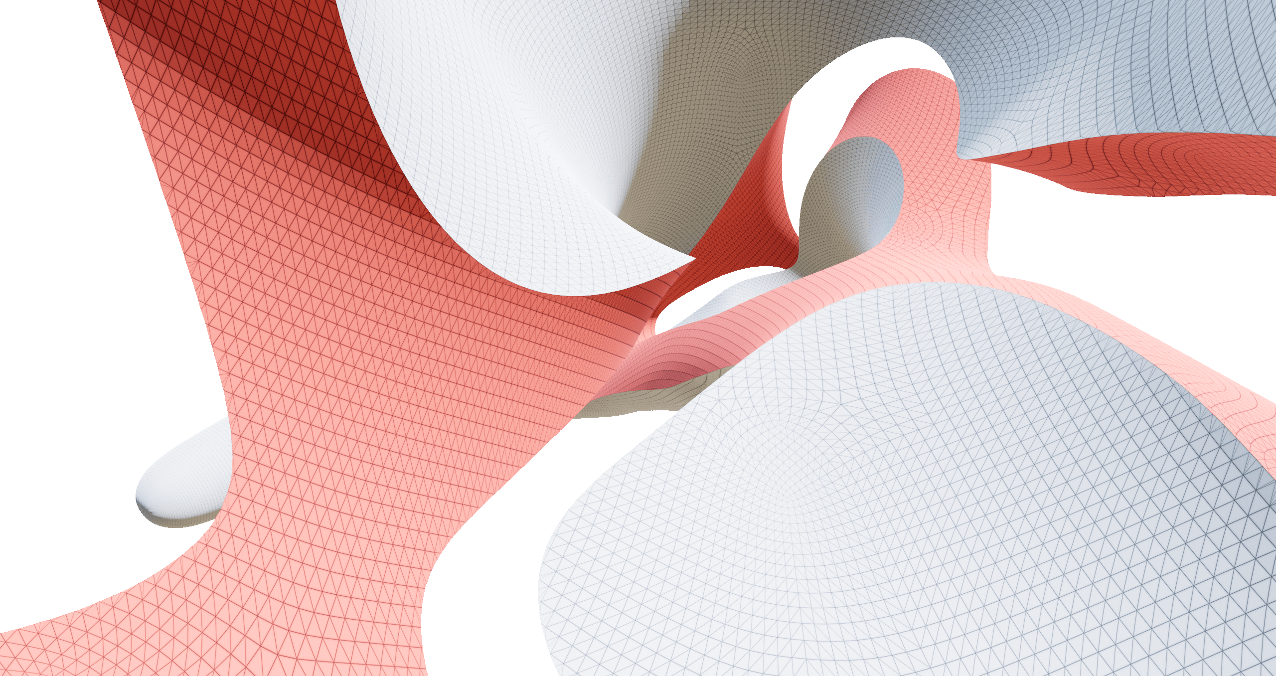
3.67 million vertices, computed in 9.78 ms (RTX 2080)
The Headache With Triangles
CSG - Constructive Solid Geometry - centers around the concept of solid masses. Whatever you do, you will need inputs and intermediaries which have a clear concept of inside and outside. Meshes are in essence nothing but a bunch of triangles (or other polygons) which can happen to properly enclose a solid, but just as easily have holes, overlapping surfaces, self-intersections, or more complex defects which violate this property.
Avoiding the deep dive here, meshes - “boundary representations” in CSG terms - have defects so plentiful, easy to run into, and hard to detect or work around, that most heavy-duty, production CSG solutions focus on a different paradigm for representing solids, “volumetric representations” being a prominent example. Think a voxel grid, each cell storing a binary value: It’s either part of the solid (inside), or not (outside).
Meshes have additional problems: Unlike voxels, they are harder to locally access and modify, both on a data-logistical level, and because local modifications can easily destroy (global) well-definedness of the underlying solid.
The algorithm running live, new results rendered each frame
Some Motivation
This sounds like lots of bad news, so why bother? Triangle meshes are of course omnipresent in real-time graphics. Almost everything in the field is triangle-based. Chances are, the things in our scene we’d like to CSG-modify are already present in mesh form, and the existing rendering logic would easily process the conventional mesh output.
Additionally, meshes can have fine, sharp details without hassle and require relatively little memory - especially compared to the cubic memory cost of voxel/grid based representations.
Algorithm Overview
At a high level, we need to solve these tasks in order:
- Build an acceleration structure of both input meshes
- Intersect all triangles in mesh $A$ with all triangles in mesh $B$
- Cut up all triangles along these intersection segments into new polygons
- Classify all polygons to be inside or outside the other, original mesh
- Assemble output by keeping or discarding classified polygons based on the CSG operation carried out
With all said and done, we start with two indexed tri meshes in GPU buffers, and a few milliseconds later, end up with a new one representing the operation result. I’ve written two versions of the algorithm: One doing everything with conventional compute shaders, and one solving step 1., 2., and 4. with dedicated raytracing hardware (and -shaders) instead.
Acceleration Structure Build
To do the pairwise intersection of all triangles without dying from the quadratic complexity, we of course need some way to speed things up - varying depending on whether we use compute-only, or leverage hardware raytracing.
Compute: Multi-Pass Morton Code AABB Tree
In the compute version of this step, a BVH is built for each of our two pre-transformed meshes. Before anything else, we transform our indexed mesh into an array of triangles and compute their AABBs. Additionally, we compute the morton code of their AABB centers, after converting them to normalized coordinates in $\in [0, 1]^3$, relative to scene bounds.
// Expands a 10-bit integer into 30 bits
// by inserting 2 zeros after each bit.
uint expandBits(uint v)
{
	v = (v * 0x00010001u) & 0xFF0000FFu;
	v = (v * 0x00000101u) & 0x0F00F00Fu;
	v = (v * 0x00000011u) & 0xC30C30C3u;
	v = (v * 0x00000005u) & 0x49249249u;
	return v;
}

// Calculates a 30-bit Morton code for the
// given 3D point located within the unit cube [0,1].
uint morton3D(float3 pos)
{
	pos.x = min(max(pos.x * 1024, 0), 1023);
	pos.y = min(max(pos.y * 1024, 0), 1023);
	pos.z = min(max(pos.z * 1024, 0), 1023);
	uint xx = expandBits((uint)pos.x);
	uint yy = expandBits((uint)pos.y);
	uint zz = expandBits((uint)pos.z);
	return xx * 4 + yy * 2 + zz;
}
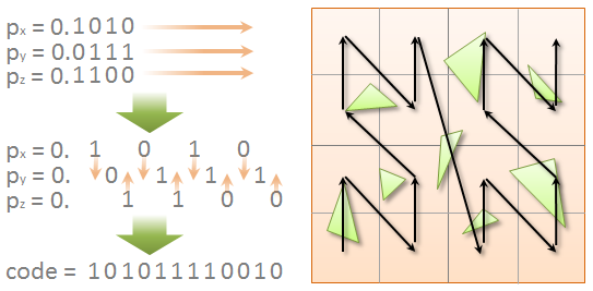
HLSL code to compute the morton code of a position
Morton codes impose a very useful linear ordering on our 3D positions, which allows for an efficient scheme to quickly build a BVH, also callad a Karras Tree, named after Tero Karras.
With the morton codes computed, we sort them in parallel with a Bitonic Sort - creating a reordered indexing instead of actually reordering the morton code array.
struct BVHNode
{
	float3 aabbMin;
	uint indexLeftChild;
	float3 aabbMax;
	uint indexRightChild;
};
Next, and without any additional geometric information, we construct a binary tree from contiguous ranges in our sorted (re-indexed) morton code list based on common prefixes. A common prefix of two morton codes correspond to the two points being “roughly in the same region”, increasingly closer depending on the prefix length.
Only as a postprocess do we insert the exact AABB bounds into our tree by propagating them bottom-up, using some atomics on a reserved flag field to avoid data races.
Finally, we end up with a BVH per input mesh which can be queried relatively quickly. To end up at this stage, we are already 6 unique compute shaders down (Primitive Build, 3x Bitonic Sort, Tree Build, AABB Propagation), the last two using recursion. Back during development, i wrote Notes on Shader Recursion covering this topic in some more depth.
Raytracing: Bottom-Level and Top-Level AS Build
For the raytracing version of this step, all of the above logic is taken care of for us by the fixed-function acceleration structure build. We simply build two Bottom-Level Acceleration Structures (BLAS), one per input mesh, and then combine them in a single Top-Level Acceleration Structure (TLAS) with world-space transforms applied. The only notable thing here is to mark the two BLAS instances with flags to allow distinction later on during traversal.
Triangle Intersection
In the intersection stage, we want to record all primitives in the other mesh intersecting with each of our meshes’s triangles, and vice versa.
Compute: BVH Traversal
Visualization of BVH nodes traversed when querying with a single primitive
With our BVH using AABBs as interior nodes, it’s only logical to once again query it with our focus triangle’s AABB again - allowing for a fast test at interior nodes.
// branchless aabb-aabb test
bool TestAABB2(AABB_CE a, AABB_CE b)
{
    float3 diff = Abs(a.center - b.center);
    float3 e = diff - (a.halfExtents + b.halfExtents);
    return e.x < 0.f && e.y < 0.f && e.z < 0.f;
}
The traversal is once again recursive, and we just require a bit of atomic logic to allocate space for our found hit IDs in the “hit array”.
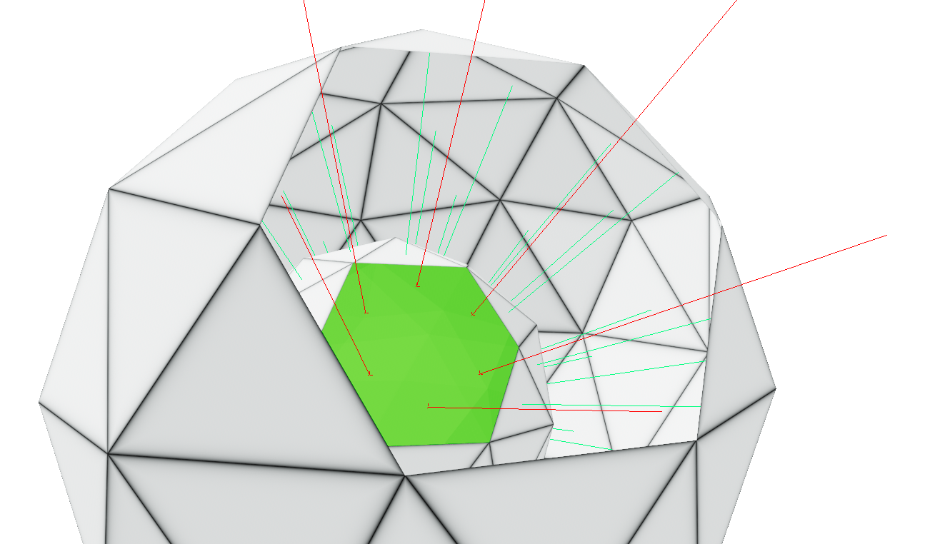
Raytracing: Triangle Edge Rays
Our RT AS cannot really be queried with an AABB, so we need to think of a different way to sufficiently query it using rays only. RT rays can be constrained with a maximum length, effectively making them segment tests. This way, we can test all triangle edges against the AS, which turns out is always enough - provided both meshes perform this check.
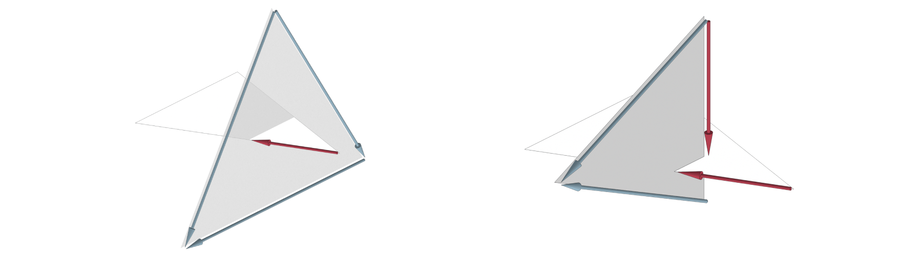
Our ray generation shader runs a grid-stride loop over the input primitives, dispatching three rays each time. We have a single-line miss shader which simply writes an invalid value to the payload’s hitPrimitiveId, and a two-line closest hit shader only recording the PrimitiveIndex() and RayTCurrent(). Back in the ray generation shader, we record the hit primitive IDs as before.
There’s a small catch here however: An intersected triangle doesn’t necessarily detect all of its intersections with its own rays (see the left example in the image above). This time, we need record our found hits in both hit arrays, the one we are generating from, and the one we traced against. Also note, this can create duplicate hits - we’ll keep this in mind for the next stage.
Polygon Cutting
So far, we did a lot of work to retrieve a list of all intersected triangles, per triangle. We now need to cut up all affected triangles in such a way that we can fully keep or discard all of the resulting polygons to form a seamless result mesh. The cutting can range from just accounting for a single intersection - splitting in two - or it can splinter our triangle into tens of new polys.
To achieve a splintering of our triangle, we first need to find all cut segments - recall so far we just have IDs of the triangles intersecting us. That much is straightforward, we iterate them, and for the first time in this pipeline, perform an actual triangle-triangle test. This is sadly a little more hassle than the beautiful AABB test above - i ported Tomas Moller’s algorithm from his 1997 paper from C to HLSL, and dedicated a 400 line file to it.
On the compute-only path, this test can also fail since the intersecting IDs only resulted from AABB checks, or the triangles could have been coplanar. In both cases, we just skip to the next one.
Extending Cut Segments
For precision’s sake, we first convert the cut segments retrieved from Moller’s test into barycentrics $(u, v, w) \in [0, 1]^3$. In most cases, these positions will not be directly on our triangle edges, but rather somewhere inside of it. For everything that follows, we need to extend them out to their full extent - either wrt. the entire triangle, or an already constrained subsection of it.
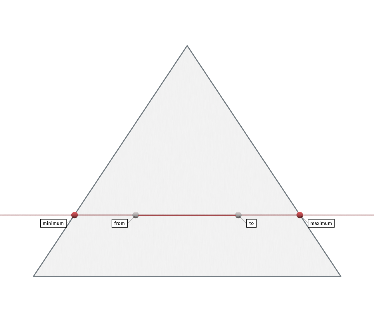
Starting with the line equation of a cut segment with endpoints $\vec{\alpha}, \vec{\beta} \in [0, 1]^3$, we rearrange its line equation $u(t) = t\vec{\beta} + (1 - t)\vec{\alpha}$, and solve for a $t^\prime$ where the first component (wlog.) becomes zero:
$$u(t^\prime)_x \stackrel{!}{=} 0 \iff t^\prime = \frac{-\alpha_x}{\beta_x - \alpha_x}$$
The solutions $t^\prime_0, t^\prime_1, t^\prime_2$ correspond to positions projected to the three triangle edges. Omitting a small detail about parallel cuts here, we now care about the two innermost results, as one will regularly be out of bounds:
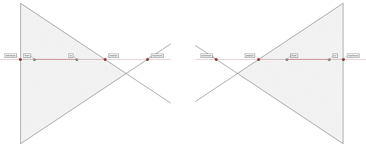
To do this, we compute the median $m = \text{max}(\text{min}(t^\prime_0, t^\prime_1), \text{min}(\text{max}(t^\prime_0, t^\prime_1), t^\prime_2))$. If $m$ is positive, one result is behind segment start $\vec{\alpha}$, and two are ahead (as seen on the left), otherwise, two are behind and one is ahead (on the right). Feeding our chosen innermost solutions into $u(t)$, we’ve got the extended points in barycentrics.
Binary Space Partitioning
A straightforward algorithm to find a correct “splintering” of our triangle given the cut segments is to use a Binary Space Partitioning (BSP). It’s another tree data structure, and this time built per triangle.
Nodes of this tree represent a splitting plane, dividing the parent node in two subspaces.
struct BSPTreeNode
{
    // v, w of the barycentrics of the segment start
    float2 barycentricsVWFrom;
    // v, w of the barycentrics of the segment end
    float2 barycentricsVWTo;
    //x: positive child, y: negative child
    int2 childIndices;

    // positve/negative meaning >0 or <0 wrt. the plane equation,
    // obtained by triToPlane(from, to, to + normal)
};
We build this tree by inserting extended cut segments one by one, recursing into the relevant subspace first, and then inserting a new node. If our segment covers both children during recursion, we also need to recurse into both of them, first dividing our segment at the splitting plane respectively.
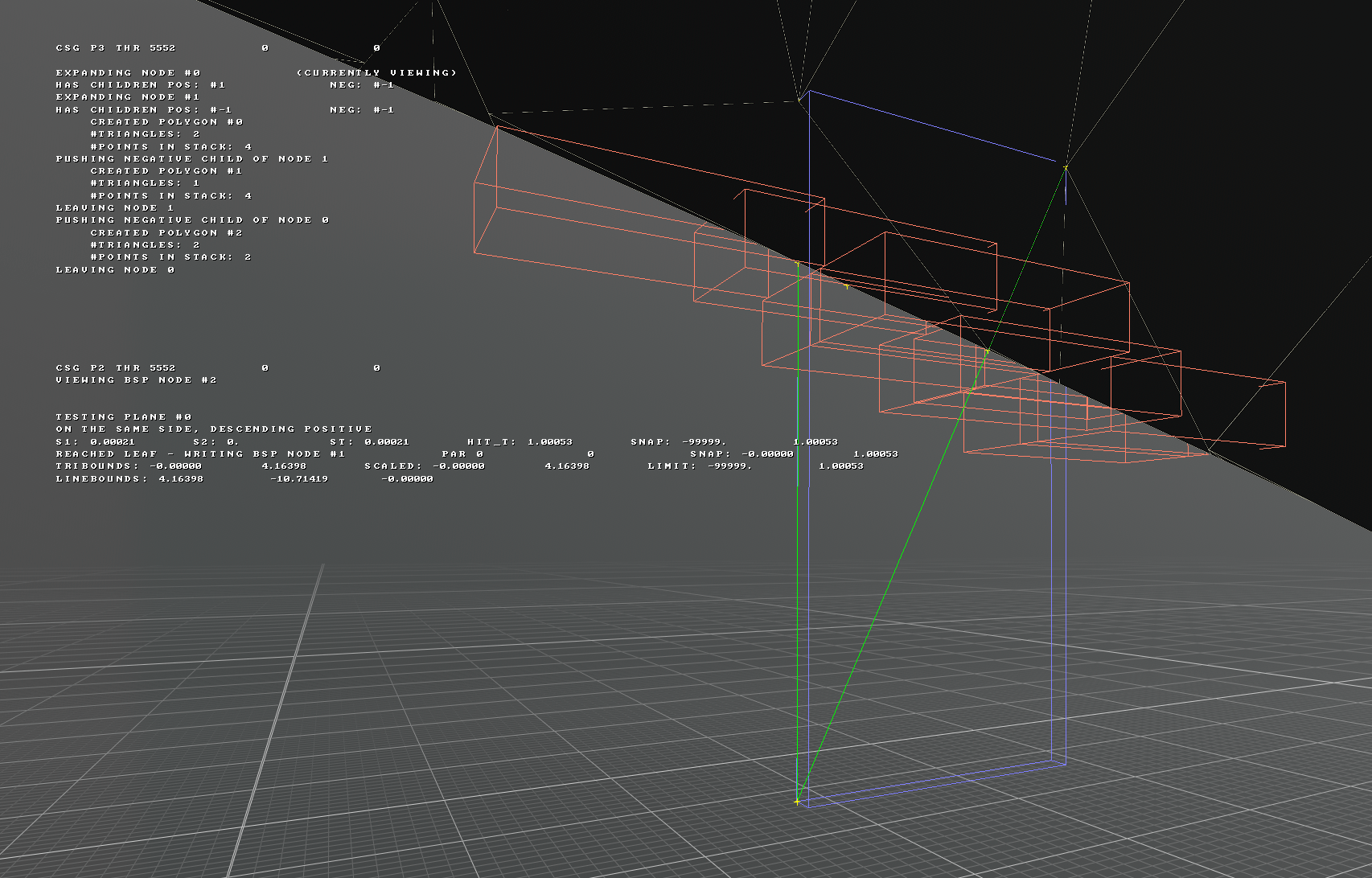
Polygon Resolve and Triangulation
After having built the per-triangle BSPs, the next pass needs to make sense of them. Their leaf nodes are plane-bounded subspaces of the triangle - polygons. We perform a depth-first traversal, storing all splitting planes of ancestral nodes in a stack $P$, as well as all “provoked vertices” $V$, meaning split segment endpoints and the original triangle vertices.
Once a leaf is reached, all vertices in $V$ are tested against all planes in $P$. If a $v \in V$ lies inside of all those planes, it becomes part of our newly created polygon, consisting of the filtered $V^\prime$. Additionally, this pass is also responsible for creating the final triangles, using a simple fan triangulation of the new poly.
To make sure we don’t create flipped triangles, we first need to sort $V^\prime$ in some manner. I decided to project them to a unit circle around their center of mass, and order them by angle - choosing an arbitrary polar point. The angle is never explicitly computed, we end up using a simpler monotonous mapping which doesn’t require transcendentals.
All of this - including the sort - takes place serially in a single compute thread (parallel over input primitives). $V^\prime$ is small - almost always less than 10 verts - and Simplesort performed just fine in my experience.
Polygon Classification
At this point, we almost made it - we have two meshes cut at their intersections and re-assembled at the seams. We just need to now throw away all of the polygons that aren’t part of the result. In this stage, we return to our acceleration structure from the beginning, and again have different implementations for compute-only and raytracing.
In essence, both versions do the same however: All polygons, new and old, shoot a ray from their center in normal direction against the other mesh, and record whether they lie inside or outside of it. The ray stops at the first hit: If it’s a front-face hit, or if it missed entirely, the polygon is outside. If it’s a back-face hit, it’s inside.
The compute-only algorithm re-uses the BVH from step 1, this time testing rays against AABBs.
// branchless ray-AABB test
// outparams: entry and exit point on ray
bool TestRayAABB(RayFull ray, AABB_MM box, out float tmin, out float tmax)
{
    // unrolled from ref: https://tavianator.com/2015/ray_box_nan.html
	const float t0 = (box.eMin.x - ray.origin.x) * ray.dir_inv.x;
	const float t1 = (box.eMax.x - ray.origin.x) * ray.dir_inv.x;
	const float t2 = (box.eMin.y - ray.origin.y) * ray.dir_inv.y;
	const float t3 = (box.eMax.y - ray.origin.y) * ray.dir_inv.y;
	const float t4 = (box.eMin.z - ray.origin.z) * ray.dir_inv.z;
	const float t5 = (box.eMax.z - ray.origin.z) * ray.dir_inv.z;

    // ray entry and exit points
	tmin = max(max(min(t0, t1), min(t2, t3)), min(t4, t5));
	tmax = min(min(max(t0, t1), max(t2, t3)), max(t4, t5));

    return tmax > max(tmin, 0.f);
}
The raytracing version of course, this time truly in its element, calls TraceRay() and records the miss, or in the closest hit shader, the HitKind() in the payload.
Output Assembly
The gathered info (polys outside or inside) is tracked in a uint array, one element per polygon, and then translated into two arrays containing “keepflags” and “flipflags” per mesh index. The actual CSG operation carried out (e.g. $A \cup B$, $B \setminus A$, etc.) translates into one of just three “modes” per mesh: KEEP_OUTSIDE, FLIP_INSIDE, or KEEP_OUTSIDE_FLIP_INSIDE.
Finally, we use Stream Compaction (as already explained in Parallel CSG Operations on GPU) to create a new compacted index buffer based on the keepflags, with the minor addition of flipping triangles whenever the flipflags are set.
All that remains is some setup for the indirect drawcall arguments to render our result in the same frame, and we’ve finally got a CSG’d mesh on screen.
In Sum
The biggest learning of this project wasn’t necessarily about geometry for me, but about building an intensely complicated and long-winded GPU algorithm. When writing a graphics effect or pipeline, you often have tangible intermediate results to look at and “get a feel for” during development, this project was a little more all or nothing.
It took getting hands on with heavy duty debugging techniques, diagnosing lots of TDRs, stepping through shaders line-by-line with PIX, staring at buffer viz, and building quite a bit of infrastructure.
As for the actual piece of tech that resulted from this - it works*, and its biggest strength is performance. On mid to high-end commodity GPUs, even very large meshes can be CSG’d within a single frame.
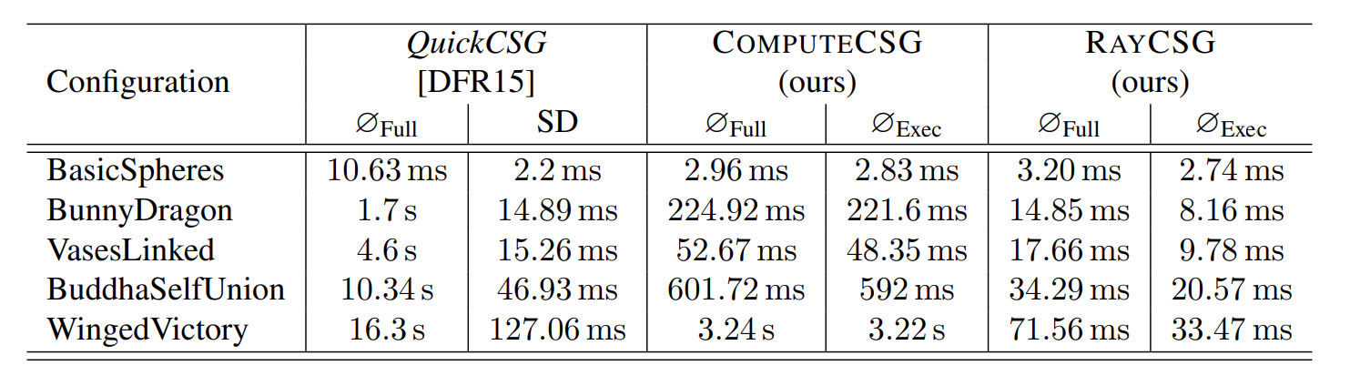
Speedups are up to 44'397 %
*However, and this won’t come as a surprise if you’re familiar with the field, the algorithm also easily falters in quite a few scenarios. To be fair, most mesh CSG approaches do, but this one especially takes few precautions against precision (float) issues. There are also multiple static limits on e.g. the maximum amount of per-tri intersections and the maximum per-tri BSP tree depth. These can be increased, but at steep VRAM costs. When exceeded, local degradations occur.
Nonetheless, it’s a fun project to look back at, even if never “shipping it”. If anything, it certainly upped my pain threshold for GPU programming.
Thank you very much for reading!